Animating in Houdini: Time-series data

Animating Time Series Data

For a while now I have been interested in finding workflows that allow me to animate geospatial temporal data through third party render engines such as Octane. I have been using Octane with Cinema4D for a while now to create abstract spatial visualisations (TopoVoxels or Topostix) but could never quite figure out how to animate time-series data… until I came across Houdini.

Houdini has been on my radar for a while, I’ve heard a lot of people say amazing things about it but always with a caveat of the ‘steep learning curve’. I decided to bite the bullet and grab the free version, since that download I’ve not stopped using it. This blog/tutorial is written from the position of a ‘self-taught noob!’ There will be workflows which probably aren’t as streamlined as they should be, or references to tools like ‘that thing that does this cool bit.’ I’ve explored so many forums and sites to try and find solutions for problems - ‘bits of python here and node configurations there’, the support for Houdini is amazing and I couldn’t have wrangled these animations if it hadn’t been for the very helpful community.

I’ve been meaning to give something back to the geospatial community for a while now, my day-to-day job in Ito World utilises bespoke software so it’s difficult for me to share workflows as that software isn’t available. So I am hoping this is useful for some folk out there who want to animate time-series data using available products.

I use a ton of different software in my workflows - driven by what I know and what gets the job done so it’s not all OpenSource unfortunately. Houdini is free to download but you are capped with a watermark and a resolution unless you purchase the indie version which is still pretty affordable ($269). I also utilise Octane as my third party render of choice, I pay for this personally as they have an amazing monthly subscription option (19.99 €) which is a pretty low barrier to entry. You don’t need Octane but most of my research into styling is through this so I’ll mention it quite a bit. You can still use Houdini’s native render engine Mantra which is still great for free.

So the following three tutorials serve as a beginners guide to understanding some of the concepts around; how to utilise time-series data in Houdini, how to reference contextual data and some basics of scene setups. I’ve based the tutorial on the above animation of bus totals in Rome throughout lock-down but you can apply the process to any binned point data. I’m also starting the tutorial from the point where by you have data or have performed the relevant spatial analysis to get some time enabled data.

You’ll also notice I start with some data in a partial array format, I am sure there are ways of getting data into this format but I utilised some of the tools at Ito to do this so can’t share workflows as they won’t be applicable. If anyone has experience with formatting data like this I can always add a prequel section to the trilogy!

Right lets get to it…

Part 1 - The Data Arrays

The concept that had me banging my head against the wall for so long was -’how do I utilise a time-series dataset in a 3d package?’ I settled on some sort of array, our Ito software utilised a similar method so I thought if I could get a series of points into Houdini with geometry and a long list of numbers relating to values at a given time I could use some node workflows to lookup an array at a given frame. Sound a bit confusing so lets look at the raw format…

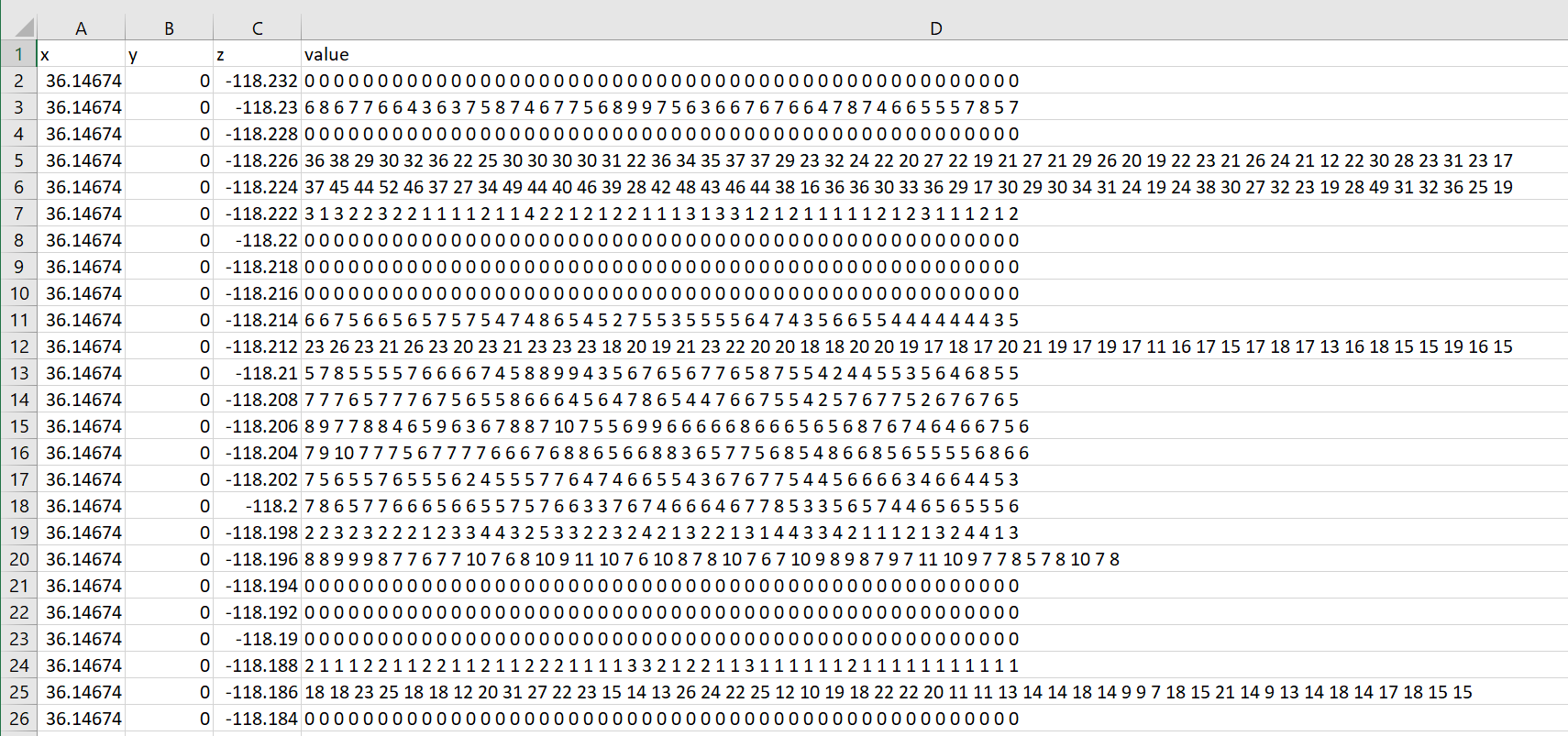
So the above data is a sample of some bus volume data. It was created using spatial binning functions, each row is a unique grid with a list of value pertaining to a specific day. First up, the coordinates - x,y,z - this is how Houdini ingests spatial coordinates, y is actually distance form the ground plane or height as opposed to z in GIS world. x,y,z refers to the centroid of the grid here, we will later use cloning tools in houdini to create a grid.

The value column, as mentioned, is a list of values by day, the index count here is 49 meaning we have 49 days worth of data. Each row has to have the same index otherwise day 30 in on row may be day 20 in another, even if a grid has zero value it needs to be present.

So how do we turn this into something we can use?

First of all this is what we want to get to, each key frame will show data for a different day, the node structure is shown on the right. Lets first take a look at ingesting that csv file.

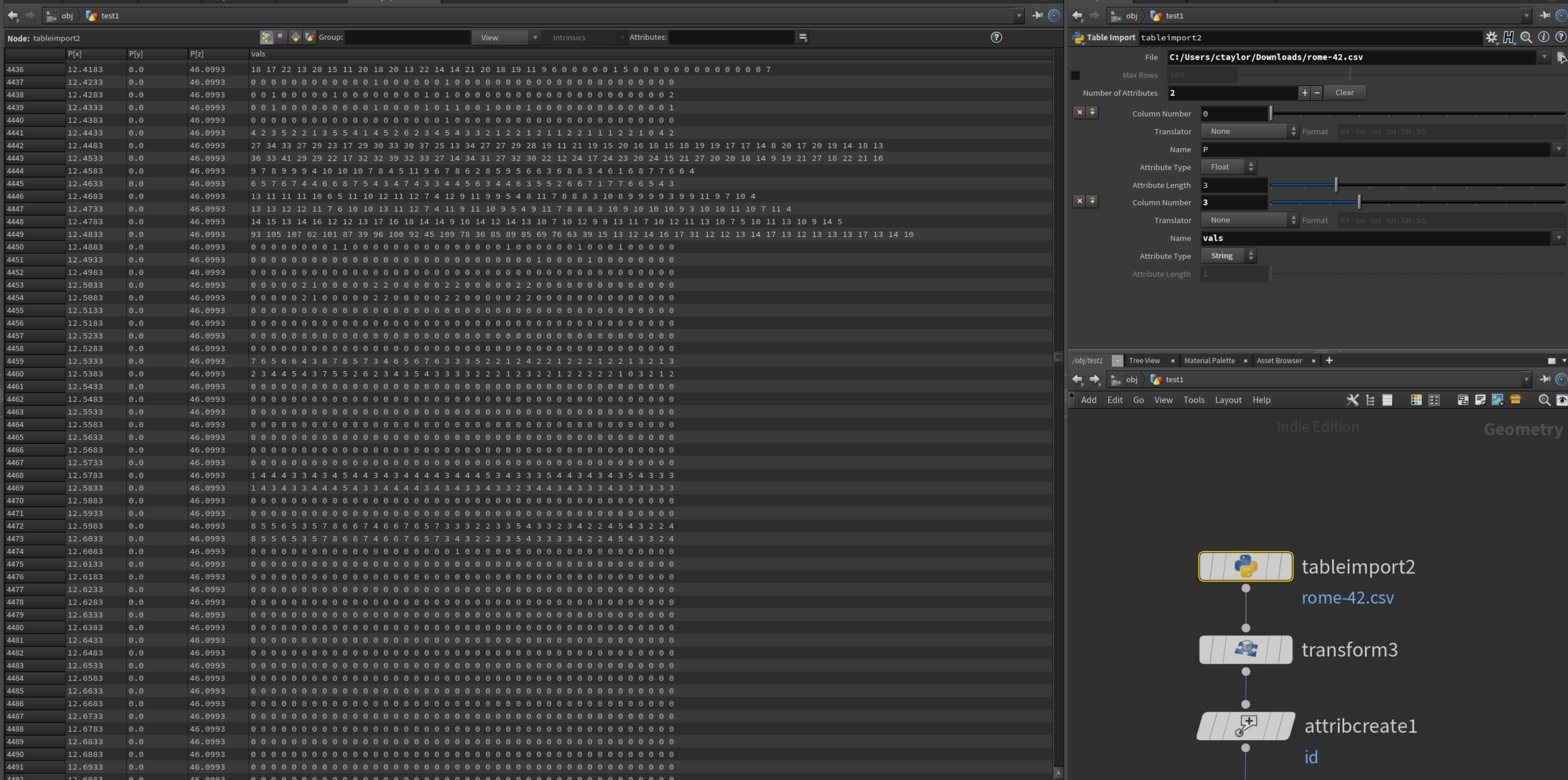
The ‘table import’ tool lets us load in a csv file and specify the nature of the columns. P relates to position and by selecting ‘3’ as an ‘attribute length’ starting at ‘column number’ ‘0’ Houdini knows to transpose the data as it is in our excel file. The next column we want to ingest is our array column, column number 3. You need to make sure the ‘attribute type’ is ‘String’ here, I’ve called it ‘vals’ for ease. If you look at the Geometry Spreadsheet view you can now see the position and array values have been loaded correctly.

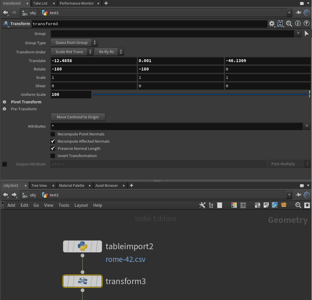
The next step is to shift our data into the centre of the viewport. You can use ‘transform’ nodes to do this easily. If you click ‘Move centroid to origin’ it does a pretty good job of shifting your points to the origin of your viewport. I’ve elevated them slightly on the ‘y’ so they don’t intersect my ground plane. I’ve also had to do some manual rotations as my data came in back to front, hence the ‘180.’ You will probably also need to scale your data quite a bit so it’s not too small, i.e. my raw coordinates were in wgs decimal degrees.

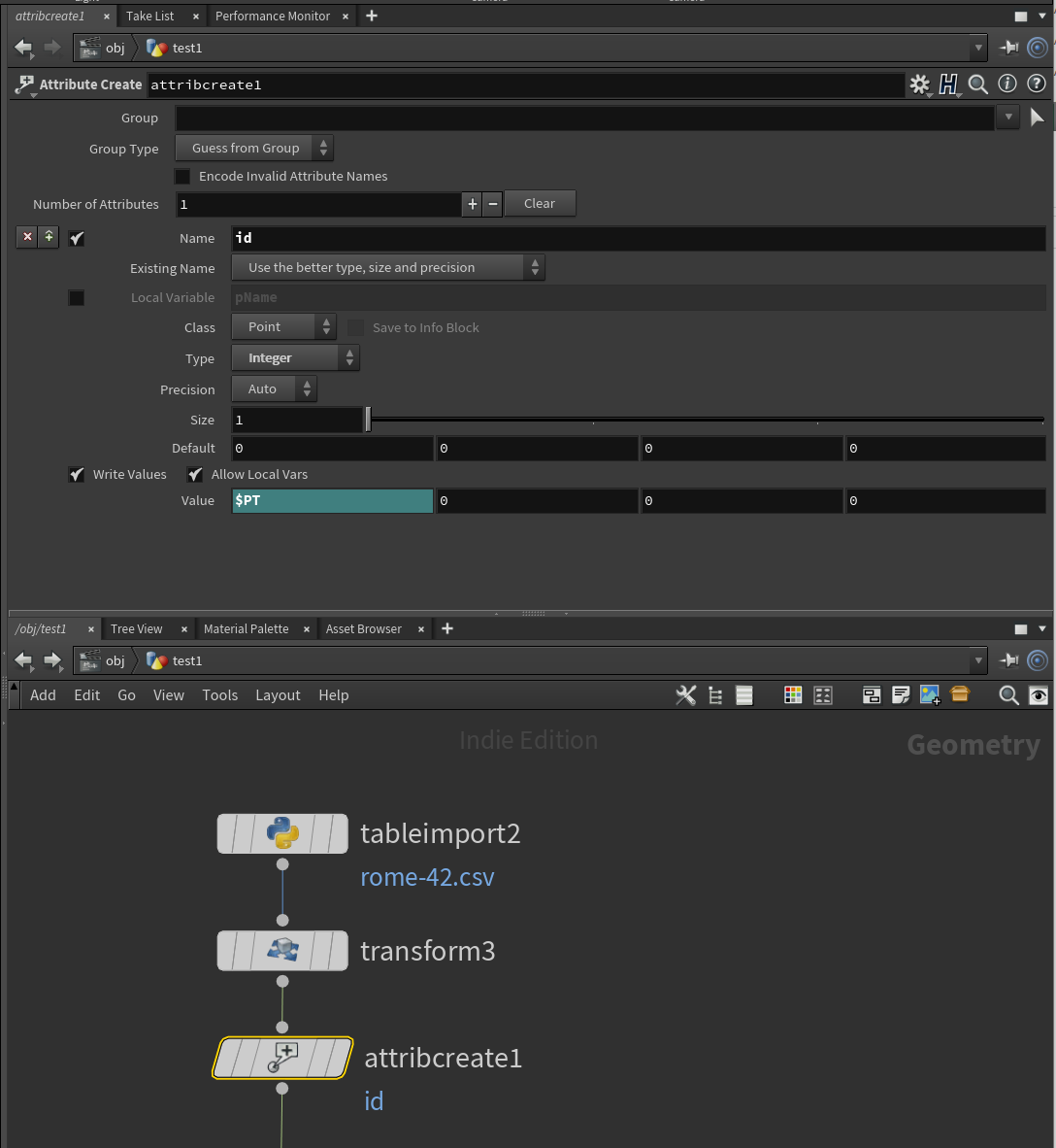
Attribute create is another useful node, you’ll have noticed I forgot to add in a unique identifier for my data, replicating these values above and adding in $PT in the ‘Value’ box will give everything an id according to it’s row.

This is where is starts getting interesting! We need to convert our string array of ‘vals’ into a Houdini recognised array so we can extract index positions from it. This requires some python and for me a lot off googling. I’m not great at coding but was able to manipulate some other examples on forums to get the array format I needed.

float @numbers[];
if(@id >= 0){
    string str1 = pointattrib(0, "vals", @ptnum, 1);
    string str2[] = split(str1);

foreach(string asdfg; str2)
    {
    push(i@numbers, atof(asdfg));
    }
}

You first need to place an ‘Attribute Wrangle’ which lets you put in the above python code. This code creates a blank array called ‘numbers’ and iterates through each ‘id’ to format the ‘vals’ string values into float numbers separated by commas in a typical array format.

Ok great, now we have an array, now to extract the values at a given index.

There are a couple of ways to extract an index number. You can create slider floats in your ‘Attribute Wrangle’ where you keyframe different index at different positions as per the below.

But I prefer doing this according to my frame number, introducing the ‘Attribute VOP’.

‘Attibute VOPS’ as far as I am concerned are like nested sub procedures, they are like a set of nodes within a set of nodes that drill into your data a bit deeper. Lets look at ‘frame index’ if you double click on this you will be taken to the VOP environment.

This looks confusing but it’s actually doing something pretty simple. Firstly we are using some nodes to convert the frame number into a float value. The purple binds are ways of either writing new data to your data-table or referencing existing data. You can use a ‘Bind’ to reference an existing column, in this case ‘numbers’, our array. Important - you need to set the ‘Type’ to ‘Float Array(float[])’ here for it to recognise the float. We then use a ‘get element’ node to plug in the array and the index (frame). This will give us the value in the array. We then use a ‘Bind Export’ to write that number to a new column. Now whenever we progress our frame the values change, the beginning of our animation!

Inevitably we will have a lot of redundant geometry that has a zero value, we can delete this by using a ‘delete’ node. We need to make sure we use ‘Points’ as the entity. Its worth noting the different levels of geometry that exist in Houdini. Up until now we are working on a ‘Point’ basis, nodes, vertices etc, any function that requires us to edit or manipulate this data is on a Point level. However when we come to creating extruded polygons we need to be aware that some of our data needs to be shifted from Point to Primitive. Back to deleting! Make sure the ‘Operation’ is ‘Delete by Expression’ and our expression is ‘@height > 0’ this should get rid of anything with 0 associated with it.

Right lets make some shapes. We can use the ‘copy to point’ to copy geometric shapes to points! I’ve assigned a circle here but changed the sides to 4 just to make the geom less complex for the time being.

Now some colour! We need to add in another ‘Attribute VOP’ here and create some functions to assign colour to the squares. We use a bind to reference our index value ‘height’ and use a ‘fit’ node to resample the value on a scale 0-1. By doing this we can put it through a ‘ramp’ node where it will associate a unique colour of any gradient you chose to the data. Note that you need to attach the ramp to the ‘Cd’ nodule in the geometry output table. Colour is generally referred to as Cd in Houdini world…

OK before we get to the 3d part we need to promote an attribute from Point to a Primitive. When we use the extrusion nodes they can only reference values in a primitive form so we are essentially copying and pasting values from points to primitives. We do this using the below settup for an ‘Attribute Promote.’ ‘parm’ in this case is the same as my height value I just created a new field in case I needed to alter the original.

Now to make it 3d!

‘Polyextrude’ is a great tool for, as you may have guessed, extruding geometry, but there are a few elements we need to understand about the node before we use it. ‘Distance’ refers to the general height of extrusion. If you go to the ‘Local Control’ drop down we can see options for a ‘distance scale’ this is where we will reference out promoted parameter ‘parm.’ Doing so extrudes the pillars in accordance with their values, you can increase or decrease the overall scale using ‘Distance’.

Scrubbing along the timeline will now alter the height of the polygons according to the index and is the basis of our animation. However we need to look at a few more nodes to fine tune the colour settings and also to interpolate our values.

Part 2 - Smoothing

So let’s quickly review what we have: An animation that has extruded pillars whose data values are linked to the animation frame we are currently on. You can think of each frame as a day. This is great but an animation of 46 frames at 30 frames a second isn’t going to last very long. We need to find a way to expand this and also to interpolate the values from one day to another. You’ll notice in my animation the pillars gradually animate up and down, there is no snapping from one value to another. Of course we assume a linear interpolation here but it’s far more aesthetically pleasing to show this interpolation than not.

Introducing the ‘Retime’ tool!

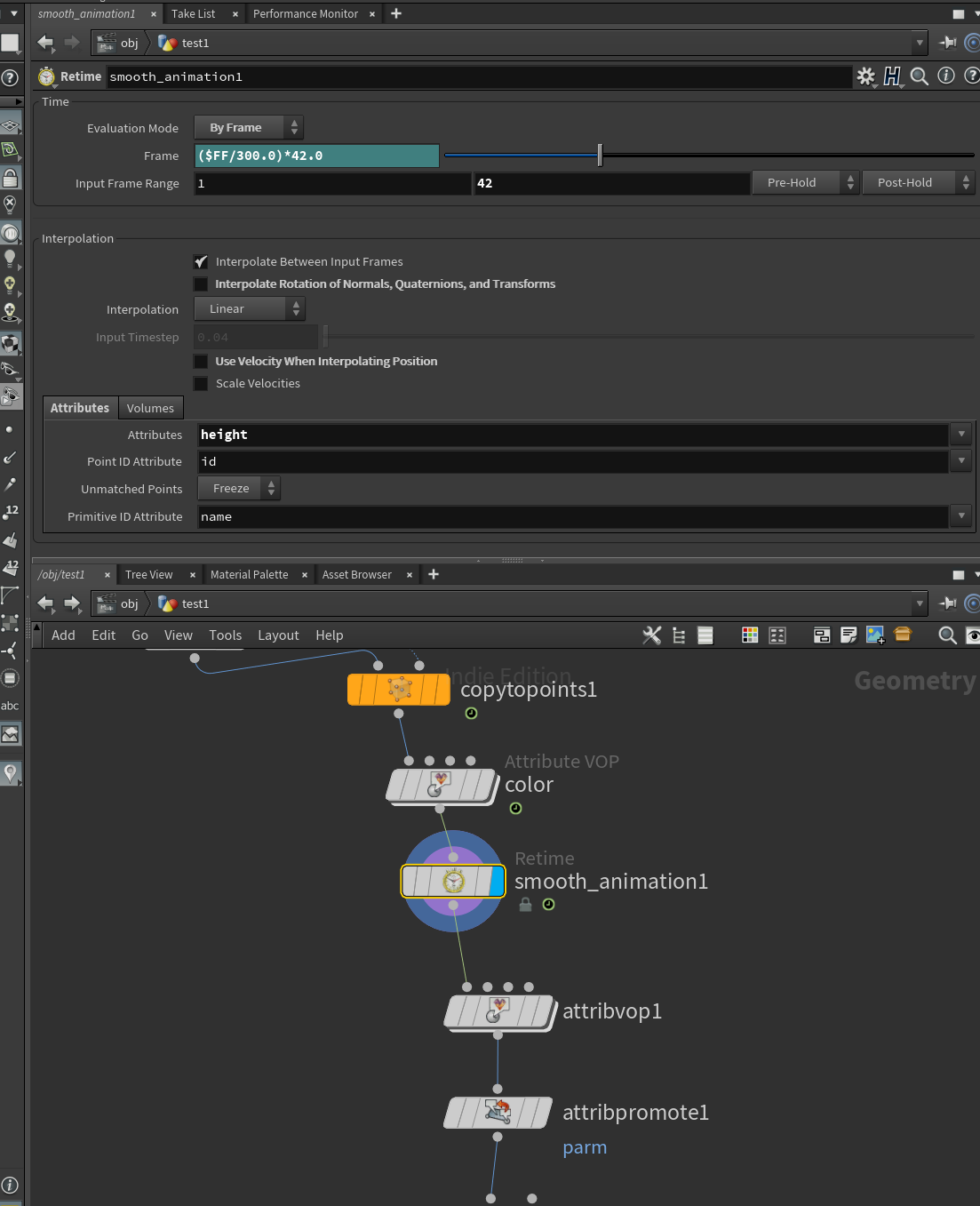
The retime tool will essentially smoothly interpolate our animation over 300 frame creating an animation which was originally 46 frames into one worth 300. So firstly stick this reference into the ‘Frame’ box ($FF/300.0)*42.0. 42.0 relates to our maximum index number and 300 relates to our maximum frame number. The ‘input frame range’ will be 0 - 42. We need to reference some attributes here, ‘height’ being the ‘Attributes’ and id being the ‘Point Attribute ID’. Once you have input all these scroll your timeline along and you should see changes happening all the way to the 300 frame mark.

Part 3 - Styling

There are a couple of ways of applying colour to the pillars, the first is as we have already done, apply a block colour to the whole of the pillar. However I prefer a smooth gradient along the vertical pillars, I feel this looks more subtle when animating. I have figured a way to do this nicely but it took some trial and error.

Firstly we need a new set of ‘Attribute VOP’ nodes for this new gradient.

Inside the ‘Attribute VOP’ we have to access the height of the pillar. We do this by converting the vector to a float ‘vectofloat’. fval2 extracts the y values (the height) of the pillar and from there we can stick it into a fit node to put the values on a scale 0-1. As per the previous example we can then put another ‘ramp’ node in and attach that to a ‘bind export’ called Cd. The colour will automatically be referenced and added to the pillars. But it looks weird right… the colours don’t look like they are interpolating correctly. It took me so long to figure this one out and it’s so simple, for the solution we need to go back to the ‘polyextrude’ node.

There is a Local Control setting called ‘Divisions Scale’ which subdivides the pillars into smaller geometries. If we reference in the height or parm attribute (parm was a duplicated field for height I created) we can subdivide the pillars according to their height so they are even. This, funnily enough, fixes the gradient issue!

Part 4 - Wrapping up

So lets just have a look at the whole node workflow one more time…

I hope this was fairly clear - Houdini is a bit of a beast in terms of the attention details within nodes etc. It took me a lot of trial and error to figure some things out so I have undoubtedly missed some things in here, or maybe I haven;t explained things properly. This is also the first tutorial I have written so it would be great to get some feedback as to whether the written blog is useful or a video discussion would be better?

I’m going to continue the tutorials in two more parts. Part 2 will talk about how to add in contextual spatial data whilst Part 3 will talk about some of the render/lighting settings used in the final compositions.