Animating in Houdini: Building Growth

Getting the data

The data we will be using is building footprints. For this example I am using a selection from Portland, Oregon via http://gis-pdx.opendata.arcgis.com/datasets/building-footprints . This data has ‘Year Built’ which will determine when our building will start animating and ‘Avg Height’ which we will use as a proxy for the extrusion of the building.

Formatting the data:

I will use QGIS to format the data as it’s free and open source. Formatting the data is a little tricky as Houdini doesn’t have an nice spatial importer yet. So much like one of my previous tutorials (https://mapzilla.co.uk/tutorials/houdini-contextual-data), we have to turn the data into something readable via Houdini i.e. csv.

We need each building to have a unique id, ‘Bldg ID’ will work and already exists in the attributes. We then need to extract all the nodes or vertices from that shapefile for each building so we have a list of coordinates. We will then take them into Houdini and connect them up to form polygons. Annoying, sure, as it creates large csv files, but it works…

So…

1) Load into QGIS and reproject to a better CRS, I’ve just UTM Zone 10 (N) here. This is a big dataset so you might want to extract a smaller sub section to work with. Export the selection and delete some of the redundant attribute fields, we only need ‘BLDG_ID,’YEAR BUILT’ and ‘AVG_HEIGHT’ and make sure to export into your designated CRS.

2) We then need to turn the polygons into a list of vertices, use the ‘Extract Verticies’ tool to do this and save your new point based shapefile. At this point you have some redundant fields relating to the vertex tool in your attributes, delete these part from the ‘vertex_ind’ to keep our csv file size to a minimum.

3) Add two new fields to the vertex dataset as ‘x’ and ‘y’ and calculate these coordinates using: $x and $y. Depending on the extract size this might take a little while. Your final shapefile should look similar to the below. Export this as a csv.

4) While we are in QGIS we can also create our road layer to help us orientate in Houdini. I have just used https://export.hotosm.org/ to quickly extract some road data for Portland in shapefile format. Using exactly the same method as the above we need to give the road paths a unique id if they don’t already have one, perhaps using ‘row_id.’ Then use the ‘extract verticies’ tool to extract the points in the road layer. We then create two new x and y fields and calculate the coordinates for this making sure we have exported it in the same CRS as the buildings. It should look similar to the below:

OK now we are ready to take this into Houdini land!

Importing to Houdini:

Houdini is a fairly complex piece of software so the below assumes a base level of knowledge or what the different panels to i.e. geometry spreadsheet or object viewer.

1) Create a blank ‘Geometry’ call it ‘buildings’ and double click to enter the node.

2) Add a ‘table_import’ and select the newly created building csv file. Switch to ‘Geometry Spreadsheet’ panel so we can see if we applying the correct fields. First of all delete the default column which specifies the ‘P’ or position, we want to manually add this later. So we need to add the fields in the original shapefile using the column number. So first lets add the ‘id’ which should be column 0. Make sure you set the ‘Attribute Type’ to ‘String’ and label it ID. Next lets add the ‘Yeah Built’ set the type as ‘float’ column as ‘1’ and ‘length as ‘1’. Do this again for height, x and y making sure they are all floats with lengths of ‘1’. This is a bit of a faff but once it’s done we should be good.

2) Step 2 is to assign the x and y field to the actual point geometry. To do this we use an ‘attribute vop’ this lets us convert current positions to floats and add or ‘bind’ existing attributes to these values. You can see the layout from the below, we first use a 'vec to float’ which seperates our xyz coords, we then add ‘binds’ for x and y. A bind is basically a way of importing other attributes. I then add these binds using an ‘addition’ node and plug them into the opposite nodes in a ‘float to vec’. Sometimes x and y get muddled up so you need to flip them around. Plugging this ‘float to vec’ into the ‘P’ socket of the geometry output will assign our coordinates.

3) Part 3 is adding a transform to move the data to the centre of our viewport. You can automatically calculate that in the transform by clicking ‘Move Centroid to Origin’, if you have no ‘null’ vales in the coordinates it should do a good job of centring your data. You may also want to scale down or up depending on the size of the scene. In this case I have scaled by a factor of ‘0.2’. One note about float precision, you always want to project your data into metres, point precision for zoomed in areas using decimal degrees can mean that you end up generalising too much.

4) Ok let’s turn these point into polygons. Place an ‘add’ node and in ‘By Group’ check the ‘Attribute’ drop down in the ‘Add’ option. In the ‘Attribute Name’ write ‘id’, this relates to our id column so if you have called it something different change it to this. Make sure to check ‘closed’ too and, voila, out points now become polygons.

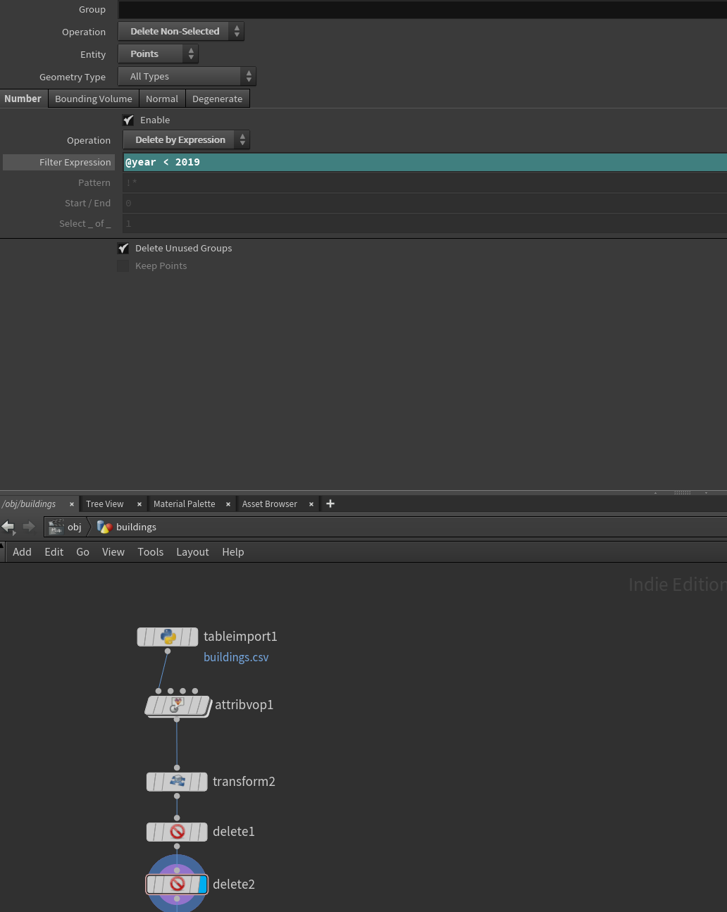
5) Removing erroneous years. So for me there were some null values in the year column which we need to remove. Use a ‘delete’ node and make sure you have the ‘Entity’ set to ‘Points’ and the ‘Operation’ to ‘Delete by expression’. Add this in the filter: ‘@year > 1800’ and check ‘Operation’ at the top is ‘Delete Non-Selected’. Add another one of these and in the filter add ‘@year < 2019’. This makes sure that we have no erroneous values.

6) Right now for the tricky part, we want to utilise the ‘year’ column as a proxy for when the builds start to rise, we don’t just want them to appear we want a gradual increase over time, something that we can alter. There is a bit of maths here, I am not great at maths but managed to cobble together a workflow than seems to work! Start bny dding a new ‘attribute vop’ after our ‘delete nodes.’

6a) Lets start with how we will drive the animation and the easiest thing to do is via the keyframe or timeline, our animation will be 300 frames long, so at 30 frames a second we will have 10 seconds of animation. We need to use a method that passes the keyframe number into our attributes using ‘in to float’ from the Frame socket. We will then divide this by our total frame number 300 and negate and multiply it so we have a value going from ‘0 to -1’ over the span of 300 frames. Notice how below I use a ‘bind_export’ if at any point you are unsure what the output is stick one of these in and it will write your value to the attribute table so you can see.

6b) Ok now to sort out what that keyframe will drive. So we have our year column and I think with this data it spans from 1846 - 2018. So we first need to bring in our year column via a bind. Then we need to subtract the lowest year from the dataset i.e. ‘1846’, We then want to divide that number by the now maximum year value which should be 172 (i.e. 172 days after 1846). This should put us on a nice scale of 0 - 1 for all the building years. We then use our frame output and add that to this new standardised number as per the below.

6c) Now for more maths stuff. So from this add node we want to multiply this value by a factor, this factor controls the speed a building will reach its apex when the year is triggered i.e. how long it grows for. I’ve used a value of -20 here as it gives a nice growth animation speed. This then gets ‘clamped’ from 0-1 and then goes into a ‘power’ node with an exponent of 0.5. So this value is our ‘height’ multiplier and will be used in a ‘multiply’ node with our building ‘height’. As it drives from a scale of 0 - 1 when multiplied with the building height it gives the effect of a building growing from the ground. The output of this is a ‘bind_export’ node with the title ‘height2’ for lack of a better name :)

7) OK now to make stuff 3d. So we need to use our ‘height2’ attribute to extrude these polygons. First of all we need to ‘promote’ this value from a ‘point’ to a ‘primitive’ so we have a blanket value for one polygon. Use an ‘attribute promote’ node for this.

8) Then we need to use a ‘poly extrude’ tool to make everything 3d. There are 3 fields you need to keep an eye on in this node. The first is ‘Distance’, this is an overall factor for how much to extrude the polygons by. You can work out the accurate version of this by how much you scaled back you data in the initial transform node or just extrude to what you think looks good. I often exaggerate heights for dramatic effect ;) Divisions are also important as it helps distribute colour if we are adding a gradient ramp. Finally the most important is the ‘Local Attributes’ section in particular ‘Distance Scale’. We will stick our ‘height2’ attribute in here and you should see everything start to pop our of the ground. If you see nothing try skipping to a later keyframe in the timeline and you should see polygons start to grow.

9) Nearly there now, after this node I like to add a ‘normals’ node to make sure all my normals are facing the right direction, easy enough to do.

10) Now to add some colour! So there are two ways of doing this a) by a block colour for each polygon or b) via a gradient falloff for each polygon.

10a) Lets start with a block colour. After our ‘normals’ node add an attribute vop. Inside here use a bind to bring in the ‘year’ attribute. Stick this into a ‘fit’ node with the ‘srcmin’ and ‘srcmax’ the earliest and latest year respectively. You then need to stick a ‘ramp’ node in and plug that into a ‘bind_export’ node and call it ‘Cd’. This should write the colour to the polygon/points. To edit the ramp back up out of the vop and click once on the vop node and you will see a ‘ramp’ colour gradient which you can edit as per the below.

10b) The other option is to use the height of the building as a proxy for colour and not year. To do this follow the below node workflow, very similar to the version with the year although we don’t bind an attribute we just access the ‘y’ coordinate of a point to utilise as a proxy for colour.

Weird Glitch Alert : Depending on what render engine you use I was getting some artefacts with the rendering of colour using Octane. I can’t figure out what is causing it but it you add a delete node after it with the below expression it seems to fix it. Very odd!

Adding the roads:

Its entirely up to you if you want to add contextual data or not, I like to keep things simple but sometimes adding in some context can help frame a visualisation. I mentioned the process of creating the road data in QGIS earlier in this blog so I’ll quickly share the node set up to add in the road data. I also have another tutorial here that talks about this process in a little more detail: https://mapzilla.co.uk/tutorials/houdini-contextual-data

1) As per the buildings use a ‘table_import’ to add the csv data, remember we need data columns for ‘id’,’x’ and ‘y’ so add these accordingly. We then use an attribute vop similar to the building data to ‘bind’ the x and y attributes to the geometry of our points. Use the same transform node you used for the buildings to make sure everything is sitting correctly. Finally use the ‘add’ node to group linear paths by attribute ‘id’ and you should see you roads all link up nicely.

Final Touches and rendering:

I’ve decided it’s too tricky to cover the in’s and out’s of rendering mainly because not everyone uses Octane and I haven’t really used Mantra (Houdini inbuilt system) enough to really give a tutorial. If there is specific requests for how to utilise Octane and pass colour values to shaders etc you can ping me and I can give you advice. Hopefully the concept is easy enough to follow but can also be applied to any geometry and any data with a time element to it. Here are some of my recent renders and screenshots while testing the workflow, hopefully it will spark your creative juices to create some similar animations!