Animating in Houdini: Contextual data
Contextual Data
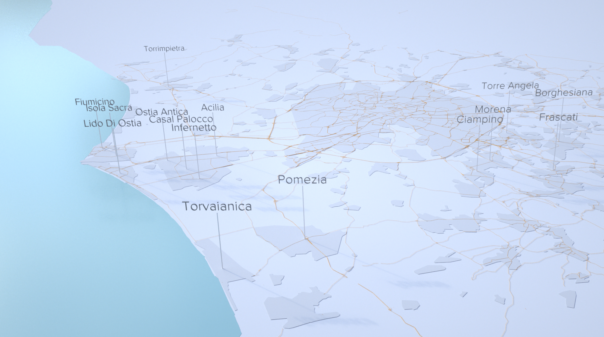
Contextual data is really important for creating a sense of place in visualisation, it allows a user to become more familiar with the geography of a particular area and as such they can appreciate and understand the data in relation to that context data i.e. is their more congestion on high speed roads or low speed inner city roads.
Therefore having the ability to populate a 3d visualisation with elements like roads, urban extents, coastlines/rivers is super useful. Unlike Blender, Houdini doesn’t seem to have many spatial plugins for you to be able to load in shapefiles etc. The ‘SideFX Labs’ shelf does offer some support for .osm files which can help but I found it a little cumbersome to turn all my data into osm files. I have managed to find a couple of alternatives which seem to work nicely.
Option 1) CSV import - involves turning spatial data into node pairs. Useful for Road geometry.
Option 2) .Shp -> .Obj - involves turning shapefiles into .obj (via blender) and manually scaling and georeferencing. Useful for land/coastline/urban (large polygon) features.
Option 1
Load a shapefile into QGIS (or similar GIS tool) and use the ‘Explode Lines’ tool to split complex lines into simple node - node pairs.
Generate a unique id for each geometry using field calculator, base it on row_id for ease.
Then use extract vertices to turn the linear path into a point dataset. This should mean you have a start and end point for each of your linear paths.
Generate x,y,z coordinates for your shapefile using field calculator. 3D can be a little different to GIS in its use of x,y,z. In GIS you often expect ‘z’ to be the vertical height off the ground place, in some 3d, especially Houdini ‘y’ is the height off the ground plane and ‘z’ would effectively be what ‘y’ was in a GIS.
Export to csv ready for importing into Houdini. You might need to fiddle around with field ordering in excel or similar, I generally find it easier for columns 1-3 to have x,y,z and 4-5 to have additional info like ‘id’ or ‘speed’. This will be apparent shortly.

Now it’s time to import the csv into Houdini, you can see the general node setup above. Table Import - Transform - (delete option for filtering fields) - Add (creation of lines). Let’s go through each in detail.
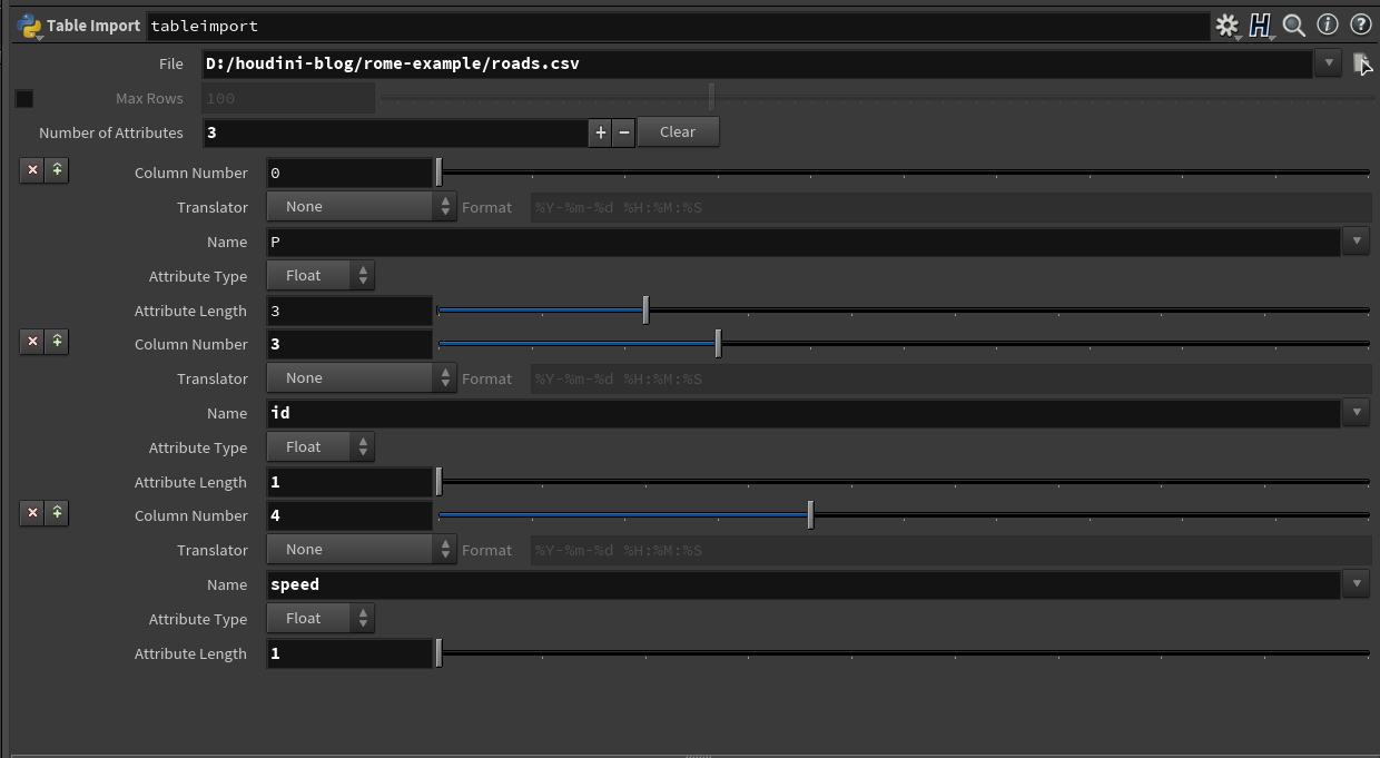
Table import

Geometry Spreadsheet View
6) Table Import. So the table import is super important to get right and can be a little fiddly with how Houdini treats certain sets of columns. For instance lets look at ‘P’ which stands for position in Houdini world. You can see that I have set the ‘Column Number’ at ‘0’ and stated it has an ‘attribute length’ of ‘3’. Selecting ‘float’ will also ensure the correct numerical type is selected, i.e. you want decimal places and not integers. The other two columns ‘id’ and ‘speed’ work in a similar way but make sure you just select that they have a length of ‘1’. Once you have replicated something similar take a look at your ‘Geometry Spreadsheet’ view to make sure that everything looks good.

Transform View
7. Transform is fairly straight forward, I used the same transformation setting we set up from the data previously to make sure the roads line up correctly. You can see I negate the x and z coordinate to bring the data to the origin of my scene and raise the roads a little so they however ever so slightly from the ground place. The rotations are needed if your data it looking back-to-front or upside down or are too lazy to put it in a format that is correct from the start! The Uniform Scale set to 100 makes sure the data isn’t too small.

Delete Node View
8. The Delete node is really useful and serves as a filter to our data, it’s optional, you might not always need to filter which is why it’s disconnected in my node setup. The important things to note here are that the ‘Entity’ is set to ‘Points’ as that’s where our attributes live and that the ‘Operation’ is set to ‘Delete by Expression’. We can then use a simple expression to filter our data according to attributes. You always need to reference a column name by using the ‘@’ sign. Common examples could be; @speed > 20 | @speed == 50 etc.

Add Tool View
9. The ‘Add’ tool is what turns our points into splines or linear geometry. Select the ’Polygon’ drop-down menu and select ‘By Attribute’ from the ‘Add’ menu and populate the Attribute name as your column name i.e. ‘id’. I’m not quite sure why you don’t need to call it using @id in this case however… Doing that will join up your nodes with the same id associated with it - creating your road geometry.
So there is a couple of ways in which you could style the road networks depending on what ‘render engine’ you are using, two options are presented below.

10a) If you are using Houdini’s standard renderer (Mantra) you need to turn the splines into physical geometry. You can do this with the ‘polywire’ node which as you can see ‘sweeps’ the splines with a physical geometry. You can set the divisions etc in the options. This is a great option but the generation of so much geometry can cause your scenes to slow down and become pretty heavy.

Octane option - fur settings

Assign render material
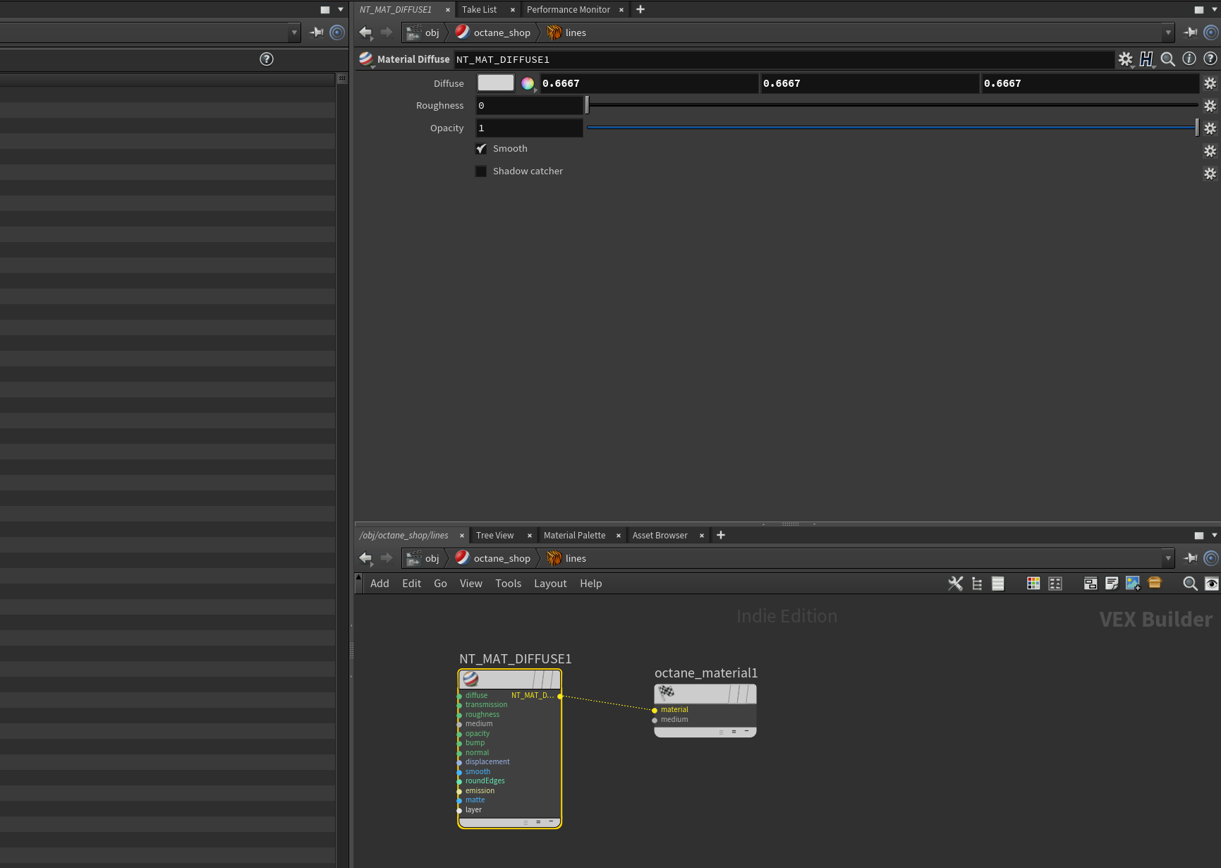
Octane material settings.
10b) So my preferred option is to use ‘Octane’, you can assign the render engine to create ‘hair/fur’ from the splines which renders a lot quicker and doesn’t create a ton of geometry. The above screenshots show how to assign this and set the width of the hair. You also need to make sure you assign the node group a material and populate the material with a diffuse/specular/glossy material.
Option 2

Rome Urban data import
So Option 2 is a little more manual in its approach, i.e. it involves manually georeferencing and scaling a 3d obj file. I am still looking into ways of importing large scale polygon data into Houdini but this methods works as an interim solution. So…
Using BlenderGIS extension import your polygon data, in this case urban shapefiles
Export that geometry into an .obj file.
Import .obj file into Houdini using the ‘file’ loader.
Using transform nodes manually position the urban extents. This is tricky without knowing where to put it on the ground, a workaround solution, although not elegant, is to convert the polygons into lines and use the same method from Option 1 to import the outline of the urban extents so at least you know where to position the obj file.
Using ‘polyextrude’ you can extrude the geometry if you want to create more of a textured 3d look and feel.
Make sure you assign a material in the node setup this time round, I had issues with .obj files not picking up materials without this node

New York grid approach
Spatial geometry, often being complex in its nature doesn’t always play nicely with 3d packages. When I first started building complex scenes in Blender for instance I found just importing large scale geometries - admin zones, country boundaries etc always used to create odd artefacts which I put down to the triangulation of the geometry. I found the best solution was to create small scale fishnet grids and run spatial intersections on the shapefiles so that when I was importing the polygons I was importing a nice set of regular grids, which triangulated more evenly. I also had this problem with Houdini, the ‘polyextrude’ tool was creating very odd glitches in the mesh for a lot of the admin boundaries. You can see how I gridded up NYC to combat this issue - only problem is an increase size in geometry!