Animating in Houdini: Scene setup

The final part of the Houdini trilogy :) involves looking at scene set up, lighting and materials. As I mentioned I use Octane as my render of choice, which comes with a monthly subscription fee. You can absolutely utilise Houdini’s inbuilt Mantra engine to light your scenes but I learnt Houdini with Octane from the get-go so I can’t really include a Mantra tutorial. So with that in mind vast portions of this tutorial might not be applicable to you but hopefully I can open your eyes to the wonderful world of Octane!

A typical scene

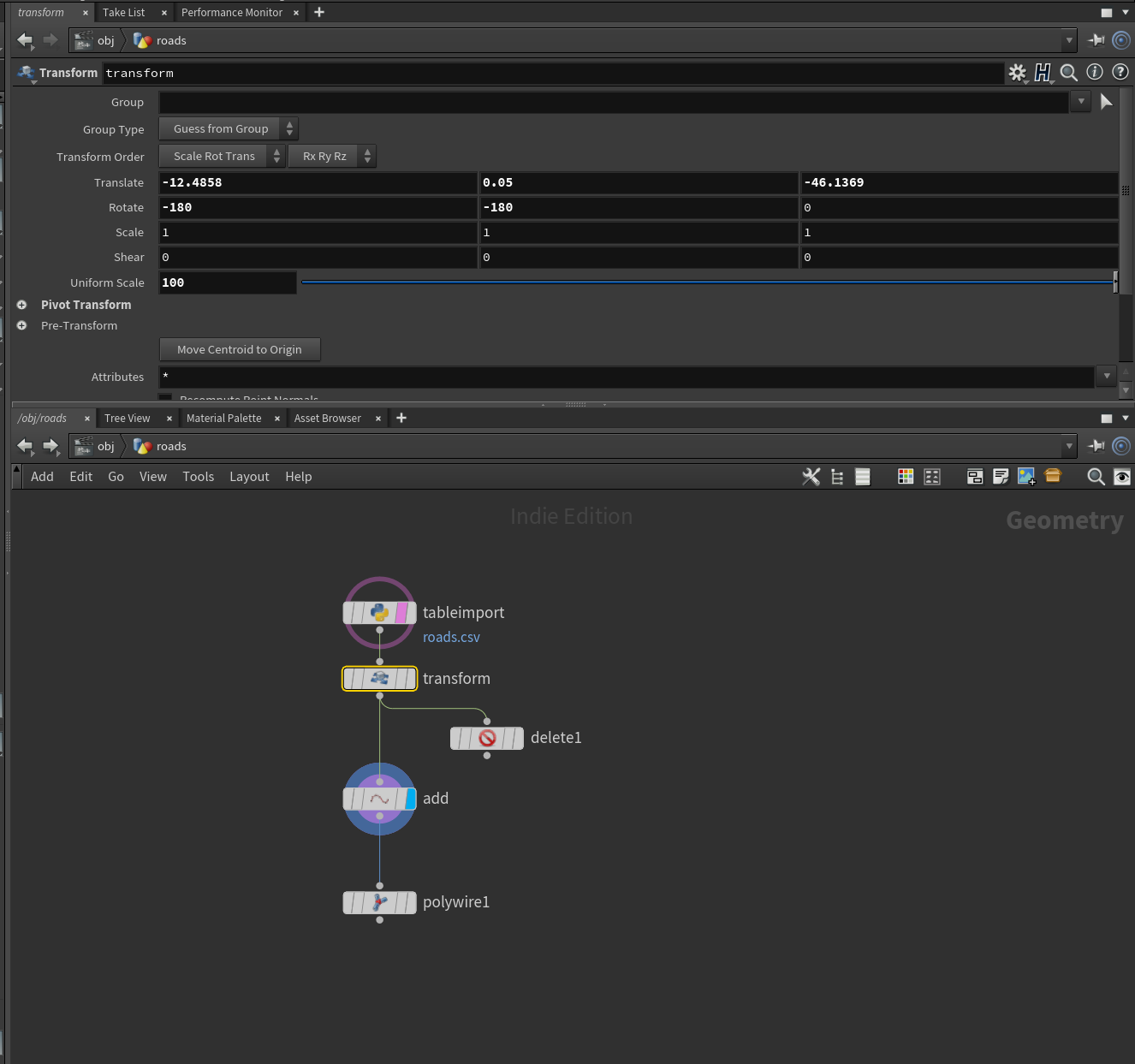
The above images shows what a typical scene looks like for me. All my nodes exist within the objects panel, each of those nodes have properties visible in the panel above it and my viewport shows what data I have visible. You can see the test1 and roads geometry nodes are blue indicating I have these turned on and are visible. The timeline on the bottom shows what frame I am on (21) and scrubbing along this will animate my data as discussed previously.

I considered doing a real in-depth description of key tools and icons but there are just too many and without knowing how relevant this is to people I’ll keep it light for now. I can always pad our the descriptions if people are interested.

Nodes

So lets talk about the classification of nodes, or node groups.

Geometry nodes:

These form the majority of the scene and hold the geometry or data for different parts of the visualisation - think of them as layers in a map. I find it easier to separate out all my layers because it’s easier to manage what is visible or what materials are assigned to each node, however you could clump groups of layers in one node group if you found that easier. Generally my visualisations are light in layer numbers i.e. the data and contextual data are minimal so I only have a few nodes.

ROP Network (render nodes):

The rop network houses the render settings for the scene i.e. where the animation sequence is output and what frames I am animating. You can see from the above settings the frames I am rendering and the syntax of $HIPNAME.$OS.$F4.png will output a filename of rome-v2.Octane_ROP1.0000.png so $HIPNAME is the Houdini file name, $OS is the render node name and $F4 is the frame number.

SHOP Network:

This confused me, a lot! The shop network from what I understand is where you materials are kept. You can see my ‘neatly arranged’ materials in the above image! Each one of these contains a subset of nodes which comprise a material - mostly octane materials. However you can also see the octane_rendertarget_dl1 node which contains more specific render settings including lighting, kernals/samples etc. I’ll go through this in more detail later.

Materials

So let’s look at a typical material for the water in our scene. First of all you need to assign a material to a geometry node. You do this via the node properties in the below screenshot.

Clicking on the water geometry node brings up the properties of that node. If you click on the Render tab you will see a Material input box, here you can select which material you want to assign to it. Now lets look at the material setup.

This is an Octane material setup, it comes with it’s own specific nodes. Here you can see I am applying a glossy material to the octane material as I want the ocean to have some reflections etc. There are a lot of options from diffuse settings to roughness to Index of refraction to tweak here.

So this process is great if you want to assign one colour to an object but what if you have an object thats colour is driven by data? Well in Part 1 we discussed the node setup to assign a colour gradient to our data. But we now need to pass that information to the material, otherwise Octane won’t know what colour to render and it will default to a pink.

What we need to do is pass the Cd to the material settings. This is done through the geometry node properties tab, within the Octane drop down you will see an option for attributes. This lets us populate some attributes from our data table to be passed to the material. You aren’t just limited to colour (Cd) you can also pass a numeric value trough the vertex attributes if you want to control opacity for instance.

Now in our material setup we can add in a Colour vertex attribute where we will reference Cd and pass it into the diffuse node ensuring that our gradient colour of the pillars is displayed correctly. I also experimented with some specular materials and passing through colour which worked nicely.

So it’s a little odd the approach of passing attributes through to materials but once you understand the workflow it becomes pretty easy to implement to other forms of data.

Lighting/Camera

Finally I just want to touch on lighting, for me lighting it one of the trickiest elements to get right, it completely dictates the mood and tone of a visualisation and is a powerful aesthetic to compliment your data visualisations. I always try to keep it simple, I don’t use lots of light probes or complex studio rigs, although I have in the past, I tend to just use a simple HDRi environment probe to get nice realistic lighting.

Within our Shop network we have our Octane Render Target settings this can be added through Octanes shelf. The settings above are my default settings, I like to use Path Tracing and my Environment is always a Texture (HDRi probe) although you can use a daylight rig in here for nice sundown vibes!

The PT Kernals tab contains your render settings for how detailed your want your scene to be i.e. samples and diffuse/specular depth. I don’t pretend to understand exactly what each setting does but best practise is to try and keep diffuse/specular and scatter depth to low values otherwise the render times for frames will be high. Samples also dictate how long you scene will render for, more samples = more of a refined image - for animation I find 500 will suffice.

I am constantly struggling to keep render times below the two minute mark but even then a 10 seconds 30fps animation will take 10 hours which is a pain. Octane has helped a lot with speeding up renders whilst retaining an amazing visual fidelity but there is a lot to be said about cloud rendering/real time rendering!

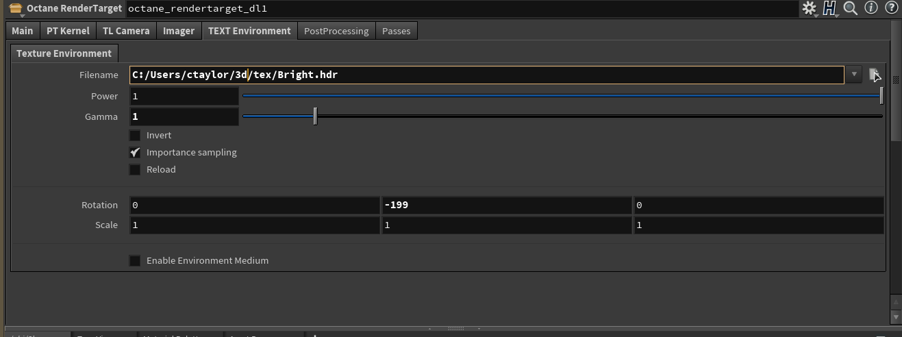
Finally the Text Environment is where you store your HDR file, rotation settings can help move your lighting around and power/gamma control the brightness and gamma of your scene.

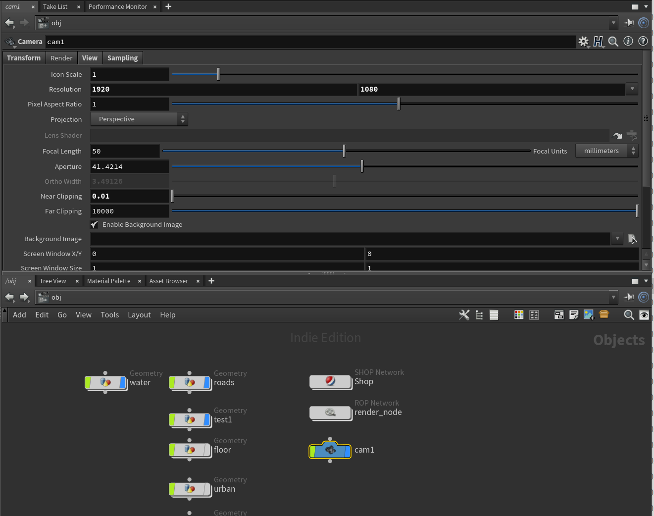
The final node of importance is the Camera node! This as your would expect frame your visualisation and contains information about the position or the camera, depth of field settings and resolution. Most settings in here are self explanatory and just require a bit of tinkering to get right.

One important aspect to note is the ability to key-frame most numeric values in the camera settings, or any node settings really. By right-clicking in a box which has a number in, camera position for instance, you can apply a key-frame which will show up on your timeline as a green bar. Moving your timeline on and adjusting the position whilst applying another keyframe will automatically cause Houdini to interpolate smoothly between the frames. There is a default easing applied to the smoothing but you can look in the animation editor to set these to a linear interpolation if your don’t want any easing curves applied.

So that about wraps up this three part tutorial series in Houdini. I apologise if any of this is unclear or I have missed elements out, it’s the first set of tutorials I have done for a self-taught piece of software so now doubt I will need to edit further! However so many people seem interested in how I am using Houdini for geo-spatial animation I wanted to at least make a start on trying to explain it!

If anyone has any questions/ideas for future tutorials please get in touch via:

twitter - @CraigTaylorViz

email - mapzillaart@gmail.com